Heat, Laplace's Equation and Random Walks on Spheres (Part 2 - the randomness)
Note: this post assumes the reader is comfortable with basic calculus and probability. The reader may skip to part 3, but would then need to do a bit more believing than understanding :)
So the stage is set. If we have our metal plate, and we know what its boundary looks like (a square, a triangle, etc.), and we know what temperature the boundary must be (imagine the flat-irons keeping the temperature at the boundary constant), then we can solve Laplace’s Equation to find out what the temperature distribution will be in steady state. Mathematically,
- We have a domain (the plate): \(D\in R^2\),
- We have a boundary (the plate’s edges) \(\partial D\in R^2\),
- We have the temperature at the boundary: \(u(x,y) = f(x,y)\) for \((x,y)\in \partial D\),
- We are looking for \(u(x,y)\), the temperature at any point \((x,y)\in D\). This function solves \(\frac{\partial^2 u}{\partial x^2} + \frac{\partial^2 u}{\partial y^2} = 0\).
(side note: you’ll notice that I’m writing \(u(x,y)\) instead of \(u(x,y,t)\) in this post. The reason is that I will be discussing the temperature distribution at steady state, wherein the temperature no longer depends on time.)
To make things concrete, let’s look at this steady state from the previous post:
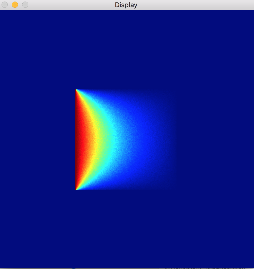
In this image, our domain (plate) is every point \((x,y)\) where \(0\leq x\leq 1\) and \(0\leq y\leq 1\). Notice that this is a square subset of \(R^2\). Our boundary (plate’s edges) is every point on the perimeter of the aforementioned square.
Our temperature at the boundary is as follows: the left wall is 100 degrees, and the other walls are 70 degrees. To be a bit more mathy, we say that our temperature at the boundary is the function \(f(x,y)\) where
- \(f(x,y)=100\) for \(x=0\) and \(0\leq y\leq 1\), and
- \(f(x,y)=70\) for \(x=1\) and \(0\leq y\leq 1\), for \(y=0\) and \(0\leq x\leq 1\), and for \(y=1\) and \(0\leq x\leq 1\).
The point in writing out these boring details is to illustrate that we can capture the temperature at the boundary with the function \(f(x,y)\).
The program that generated the above image approximated the solution to Laplace’s Equation with the input boundary conditions (the shape of the boundary and temperature along it) to find the temperature distribution in the plate. How did it do this? To find out, let us now talk about random things.
Here are our goals
- Define a random walk, and the Wiener process.
- Discuss the expectation of a function of a Wiener process.
- Use these tools to solve Laplace’s equation.
- Convert the solution into an algorithm.
In this post, we’ll address the first three goals. Coding the solution will be the topic of discussion in the next post.
What is a random walk? What is the Wiener process?
Suppose you are on a giant checkerboard, and you are standing in a square. Suppose further that, to step from your square to an adjacent (not diagonal) square, you step a distance of 1 meter. The path that you take as you step from square to square in that checkerboard (wondering how you got there) is called a walk.
Now imagine you perform this walk randomly in the following way: at every second, you decide which adjacent square to step onto by picking a direction at random. Any direction has equal probability of being selected (you could decide what direction to go by drawing a card from a deck, and heading north if it’s spades, south if it’s hearts, and so on). Here’s a picture of what that walk might look like:
There are two parameters to notice here: we’re taking a step of distance 1 meter, and we are taking it every 1 seconds. Let’s be a bit more general: in your walk, take a step of distance \(\sqrt{\Delta t}\) meters once every \(\Delta t\) seconds. In our original example, we have \(\Delta t=1\).
The Wiener process is like a continuous version of the random walk described above, and it is equivalent to the limit of the above random walk as \(\Delta t \rightarrow 0\) (think about it this way: instead of taking discrete steps, you are continuously changing direction). Here is what the 2D Wiener process looks like:

Besides being the foundation for the mathematical study of stochastic differential equations, this process also has applications in physics, finance, and more. For our purposes, it’s enough to know that it’s basically a continuous random walk. Here’s a video showing a simulation of the path taken by a Wiener process.
What is the expectation of a function of a Wiener process?
First, let’s take note of the fact that a 2D Wiener process is like a mapping which takes a time \(t\) and returns a 2D coordinate \((x,y)\) (side note: this mapping depends on where you started the process, but more on that later). From now on, we will denote the Wiener process by \(W_t\). For example, in the above video, \(W_0 = (0,0)\) since the process starts at the origin. However we must keep this critical fact in mind: \(W_t\) is a random variable, and it does not have a definite value, but rather a probability distribution (like the toss of a die, or the flip of a coin). From this perspective, you may view the above video as akin to a coin toss: it’s just the outcome of one experiment.
Now let’s remember our temperature function \(f(x,y)\) (let’s use the letter \(f\) now for a reason which will become clearer later on), which takes a 2D coordinate \((x,y)\) and returns a number representing the temperature at that point in space. What if, instead of passing a definite coordinate \((x,y)\), we talk about the temperature at the random coordinate \(W_t\)? Let us define \(f(W_t)\), to be the function which returns the temperature at the coordinate that the Wiener process (think random walker on plane) has arrived at after \(t\) seconds.
Again, this function doesn’t have a definite value for a given \(t\), but rather a probability distribution. For example, let’s say that any point in the upper half of the plane has temperature 10, and any point in the lower half of the plane has temperature -10. Take a minute to convince yourself that the Wiener process (random walker) has equal probability of ending up on either half of the plane (disregard the x-axis, the Wiener process is almost never exactly on it). Then, we have the following probability mass function for \(f(W_t)\):
- \(P(f(W_t) = 10) = 1/2\)
- \(P(f(W_t) = -10) = 1/2\)
This is shown in the following video. We let the Wiener process run for some time, say 10 seconds. Then, we take it’s value (which is a 2D coordinate) and find the temperature at that point.
Each dot corresponds to one experiment of \(f(W_{10})\). As we predicted, the result is that about half of our dots are hot, and half are cold.
The expectation of a function of a Wiener process depends on two things:
- Where does the Wiener process start?
- At what time are we taking the expectation?
For this reason, we will denote the expectation as \(w(x,y,t) = E^{(x,y)}[f(W_t)]\). Notice that \(w(x,y,t)\) is not random, but rather deterministic. Just as the expectation (average) of a die roll is definitely 3.5, the expectation of a function of the Wiener process is a definite number. In the above video, \(w(0,0,t)\), which is the expected value of the temperature at \(W_t\) given that the process started at the origin, is 0 no matter what \(t\) is (since the probabilities above don’t depend on \(t\)). If we started the Wiener process at \((0,10)\), then the expectation would be positive, but decreasing with time; after not much time, we’ll probably get a hot hit, but after a lot of time, we’re not too sure.
How does this help us with Laplace’s equation?
We’re in the home stretch now. Laplace’s equation is
\(\frac{\partial^2 u}{\partial x^2} + \frac{\partial^2 u}{\partial y^2} = 0\)
where \(u\) is the temperature inside the plate. Our boundary condition is that the temperature at the boundary (edges of the plate) is given by \(f(x,y)\).
Take a point \((x,y)\) inside the plate, and start a Wiener process at it. After a certain amount of time, this Wiener process will hit the boundary; this time is called the hitting time and is denoted by \(\tau\). Then Laplace’s equation with the above boundary condition is solved by
\(u(x,y) = E^{(x,y)}[f(W_\tau)]\)
which, in English, is the expected value of the temperature of the boundary at the hitting spot of a Wiener process that started at \((x,y)\).
Before discussing why this solution works, let us notice that the solution is an expectation of a function of a Wiener process which doesn’t depend on a time variable. This is different than \(w(x,y,t)\) above, which we used to describe the expected temperature in the hot/cold video. What happened to the \(t\)?
Without getting too formal, we can say that \(W_t\) is a random variable which describes the location of the Wiener process after \(t\) units of time, and that \(W_\tau\) is a random variable which describes the location of the Wiener process at the first time that it hits the boundary. Here is a video of many experiments of \(W_\tau\) inside a square boundary (the result of each experiment is the location of the circle. The temperatures are the results of \(f(W_\tau)\)).
This random variable has an intuitive probability distribution. If you start the random walk in the middle of a circular room, then \(W_\tau\) is equally likely to be anywhere on the circular boundary. On the other hand, if you start the random walk inside a square room, then \(W_\tau\) is more likely to be near the middle of one of the walls, and less likely to be near a corner. The location of your hit doesn’t depend on how long you’ve been walking, but rather on where you started and the fact that you’ve hit a wall. We see this in the fact that the experiments in the above video have varying times.
The proof that \(u(x,y) = E^{(x,y)}[f(W_\tau)]\) works uses Dynkin’s formula, which is a more general form of the following equation:
\(u(x,y) = E^{(x,y)}[u(W_\tau) - \int_0^\tau \nabla^2 u(W_t) dt]\)
Dynkin’s formula (which we not prove here, although we can imagine that it is like a stochastic version of the fundamental theorem of calculus) states that the above equation is true for all functions \(u(x,y)\). When we substitute in Laplace’s equation (\(\nabla^2 u = 0)\), we get
\(u(x,y) = E^{(x,y)}[u(W_\tau)]\)
Since \(W_\tau\) is on the boundary, we notice that
\(u(W_\tau) = f(W_\tau)\)
So the equation becomes
\(u(x,y) = E^{(x,y)}[f(W_\tau)]\)
And that’s the solution! It’s more general than an analytical solution, which would depend on the boundary in a disgusting way. Furthermore, it can be more efficient for finding the solution at a few points (as opposed to the entire domain) than FEM approaches. In the next post, I will talk about how a computer is supposed to efficiently evaluate this solution.