Heat, Laplace's Equation and Random Walks on Spheres (Part 1 - the physics)
Consider the following…
 Suppose I have a square, metal plate. Suppose also that I can control the temperature of each of the walls of the plate (maybe I have clamped flat irons on all four walls, and can vary the temperatures of the flat irons (don’t ask me why I have four flat irons)). I set up the plate so that every wall is the same temperature, say 70 degrees Fahrenheit. Then, at a certain time \(t=0\), I switch the temperature on the left wall to be 100 degrees Fahrenheit. Here’s a question: after a few seconds, what is the temperature in the middle of the plate? How about after an hour? And what about any other point in the plate?
Mathematically, we’re looking for a function \(u(x,y,t)\) which describes the temperature at the 2D point \((x,y)\) at time \(t\). For example, if \((100,100)\) is the point in the middle of the plate, then we know that \(u(100,100,0)=70\), by the statement of the problem (the center of the plate was initially 70 degrees). But after a few seconds, how much has the temperature at the middle of the plate increased? We’ll need to find this function \(u(x,y,t)\).
We do this by solving a partial differential equation (PDE) called the heat equation, using our initial and boundary conditions. This is the heat equation:
\(\frac{\partial u}{\partial t} = \alpha \nabla^2 u\)
where \(\alpha\) is the thermal diffusivity of the material (heat spreads differently through different materials, hence the existence of Thermos).
(side note: where did this equation come from? There are many derivations of the heat equation on the web; Wiki features a derivation in one dimension which only uses Fourier’s Law and conservation of energy. I like this, because Fourier’s Law is like a continuous analogue of Newton’s Law of Cooling, so you can imagine that the heat equation is the result of taking very simple principles that even Newton was privy to, and being very mathy all over the place)
Let’s say our plate has thermal diffusivity 1, and note that this is roughly a 2D problem (assuming the air around the plate doesn’t affect its temperature too much). Then the heat equation looks like this:
\(\frac{\partial u}{\partial t} = \frac{\partial^2 u}{\partial x^2} + \frac{\partial^2 u}{\partial y^2}\)
What are our conditions? Firstly, \(u(x,y,t)=100\) on the left wall of the plate, and \(u(x,y,t)=70\) on every other wall (we are keeping the temperatures of the walls constant). Also, \(u(x,y,0)=70\) everywhere on the plate except the left wall; this is to say that at the instant the wall is switched to 100 degrees, the rest of the plate hasn’t changed from its initial temperature of 70 degrees.
The point is, we can use the heat equation to solve for \(u(x,y,t)\), and that’s really nice. However, that’s a lot of math, so let’s let the physics undergrads work on that and I’ll get to my point.
Once we switch the left wall to 100 degrees, the heat will spread throughout the plate. After enough time, the plate will reach a steady state again, wherein the temperature of each point stops changing. If it isn’t clear that a steady state should be achieved, imagine leaving a hot cup of coffee on a table. After a minute, the coffee has cooled a bit. After 2 hours, its practically room temperature. After a day, it is room temperature. After a week, it is still room temperature - it has achieved a steady state.
Suppose I want a formula that describes the temperature at steady state at a point in the plate. Teaser: here’s what the steady state looks like:
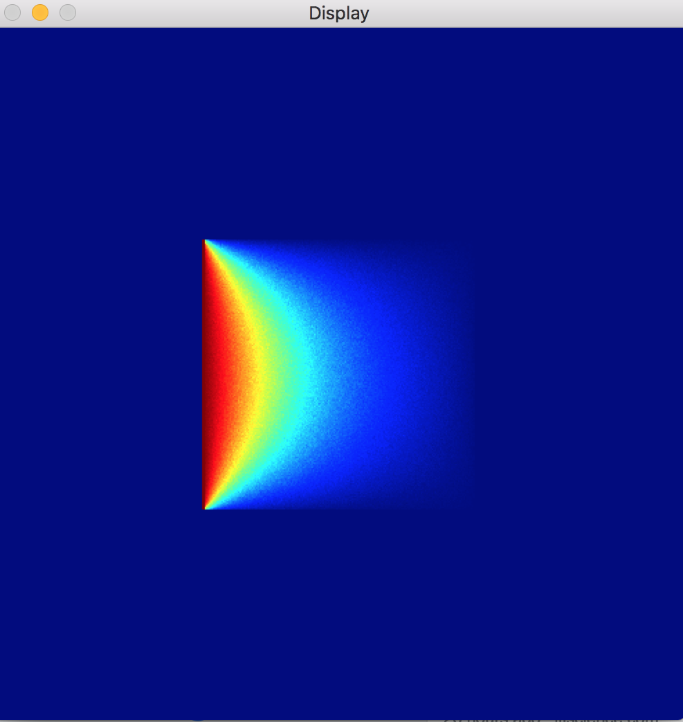
Looking again at the heat equation, we realize that, at steady state, we will have
\(\frac{\partial u}{\partial t} = 0\)
Which is to say that the temperature at any point doesn’t change with time. Then, substituting the above into the heat equation, we arrive at a new PDE describing the temperature at steady state. This is called Laplace’s Equation:
\(\frac{\partial^2 u}{\partial x^2} + \frac{\partial^2 u}{\partial y^2} = 0\)
(side note: the PDEs I’m outlining describe more processes than just the spread of heat, and can be generalized to any number of dimensions)
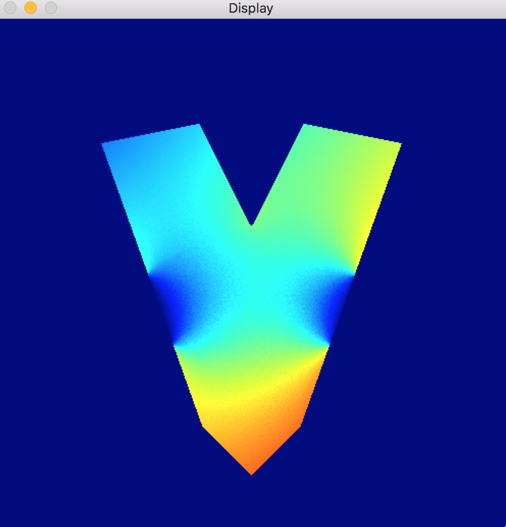
Cool, so let’s solve the PDE based on our boundary conditions, right? Well, let’s not. For our simple example, the formula for \(u(x,y,t)\) may not be too disgusting, but what if our plate weren’t square? What if our plate were a star, or a crescent, or the Mandelbrot set? Furthermore, suppose on one of our strangely shaped plates, the boundary temperature distribution were really weird? I think it’s high time we let the computers take over on this problem.
The ultimate goal here is an algorithm which, given the shape of the plate and the temperatures of its walls, finds the steady state temperature inside the plate. In my next blog post, I talk about the Random Walks on Spheres approach, which was used to generate the above image, as well as the below image, wherein the shape of the plate and the boundary temperature distribution are a bit funkier.
PS: I bought a coffee before writing this post. After finishing, I now realize that I forgot to drink the coffee, and it has now cooled. Well played, brain.